Figure 1.The Physical Oceanographic Real-Time System (PORTS) operatedin Tampa, San Francisco, Galveston and Chesapeake Bays, and in the Port of New York/New Jersey.

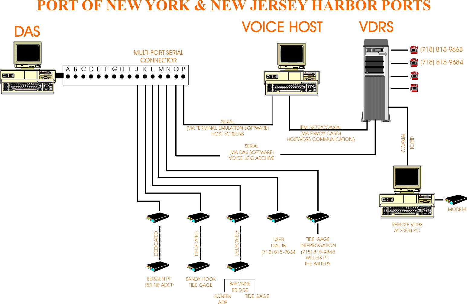
Figure 2.Schematic of the operational PORTS system for the Port of New York/New Jersey.

Figure 3.Real-time Water levels, winds, currents and water properties reported at the Boliver Roads site through the Galveston Bay PORTS system.

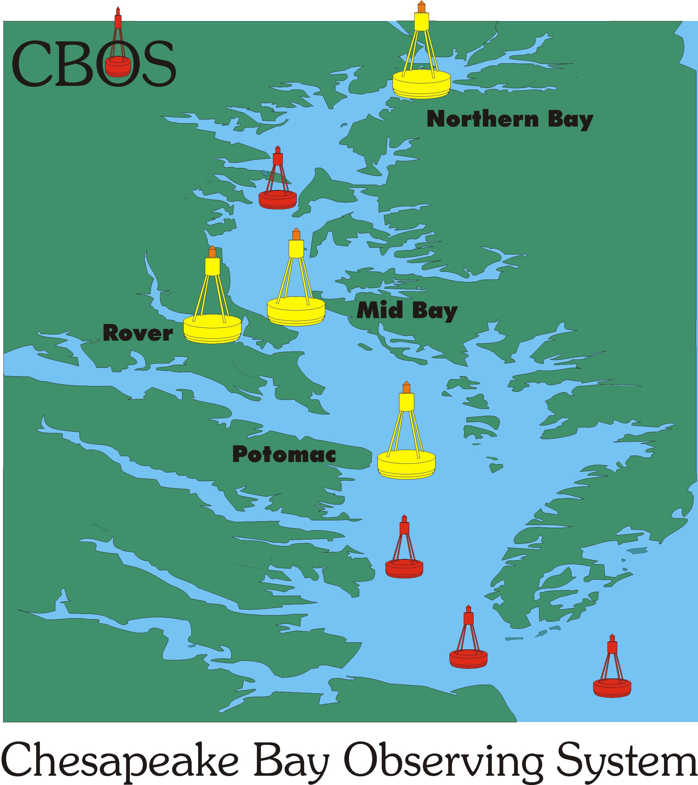
Figure 4. Chesapeake Bay Observing System. Permanent Monitoring Stations are arrayed along the central axis of the Main-Stem Bay, with four existing (yellow) and four planned (red) platforms. Rover Buoys are dedicated to research and monitoring the rivers that drain into the Bay. All buoys have individual telemetry towers on land, which communicate via the Internet to the Data Management Center at UMCES Horn Point Laboratory. Monitoring information is then processed, visualized, and released via the web (www.cbos.org).

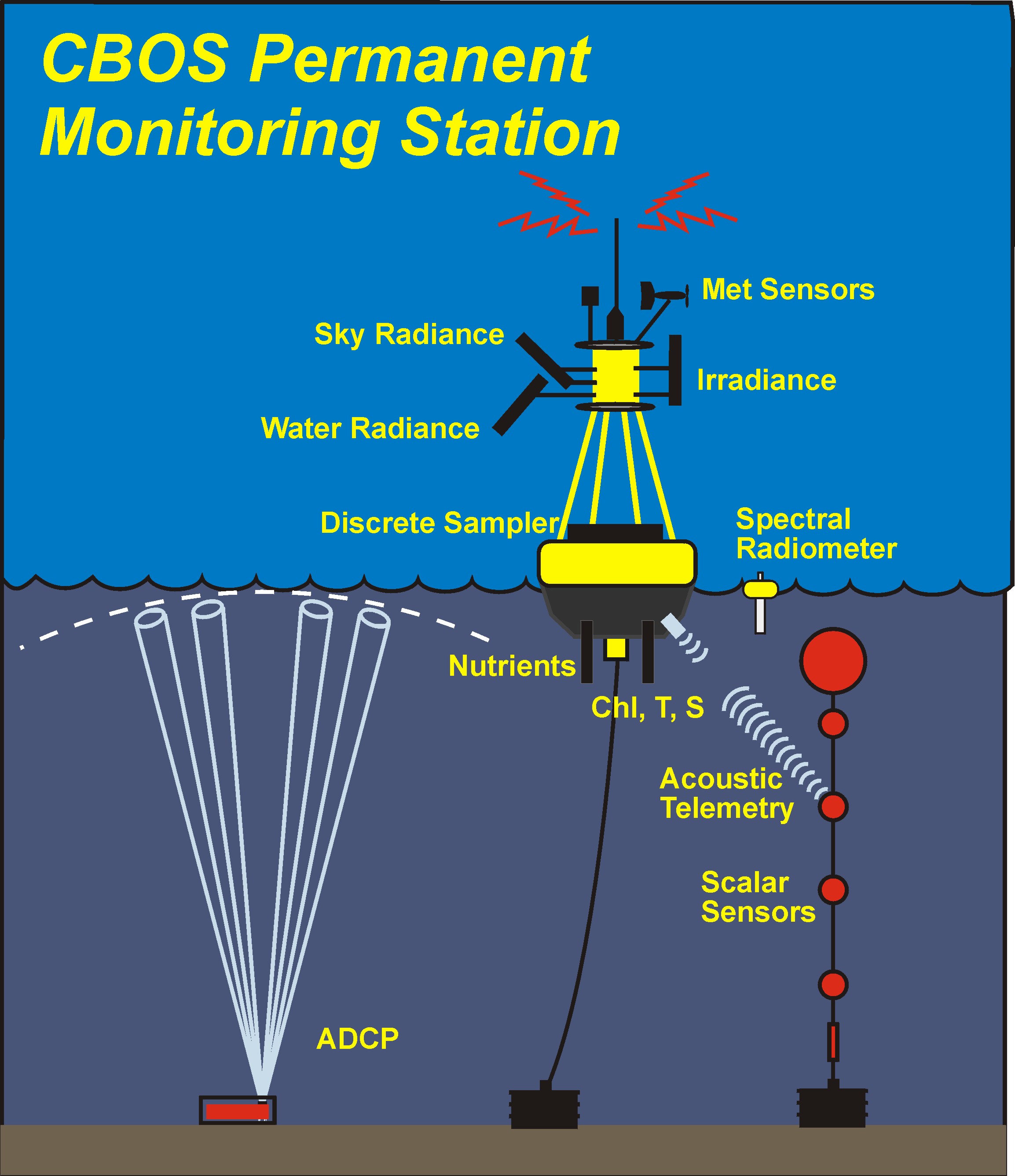
Figure 5. Schematic diagram of a CBOS Permanent Monitoring Station, showing the full sensor suite and the configuration of underwater sensor array. The surface buoy was designed sufficiently large to remain on station for one year, to allow onboard access to electronics, and to provide space for shorter-term sensor experiments. Biofouling and summer anoxia require servicing of underwater sensors at intervals of less than 4 weeks. For this reason, a separate taut-wire mooring is deployed adjacent to the surface buoy, and data are communicated via acoustic telemetry.

Figure 6: Wind forcing, water level, and subtidal axial currents from Acoustic Doppler Current Profiler at Mid-Bay CBOS Permanent Monitoring Station in summer 1996. Current and water-level fluctuations are primarily wind-driven, with the upper-layer directly forced and the lower layer responding at a lag of 12 hours to the resulting tilt of the sea surface. Low-pass filtered (34-hour) axial currents (v') are shown at 4 selected depths. Time rate of change of water level (h) at Baltimore, 100 km to the north, and relative slope between Baltimore and Solomons Island (30 km to the south of the Mid-Bay buoy) on the Patuxent River are also shown. The acceleration in lower-layer currents (21m) show a remarkable correlation with the rate of change of Baltimore water level, both during slow variations in wind forcing, and during the interval of pulsed winds that activate the 2-day quarter-wave seiche in the Bay (13-24 July).

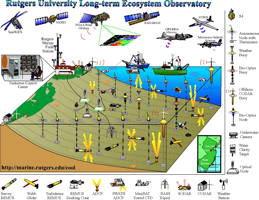
Figure 7: LEO observation network operated offshore of Tuckerton, New Jersey. Instruments shown include those used during the peak summer sampling periods.

Figure 8: LEO real-time monitoring data.Top: 1998 Bottom Temperature Time Series from LEO Node A (red) and Node B (blue).
Bottom: July 23, 1998 sea surface temperature and surface current nowcast of a fully-developed upwelling center derived by detiding and low-pass filtering the combined CODAR vector velocities. Lines indicate the locations of the three cross-shelf repeat transects chosen for subsurface shipboard (black) and AUV (red, white) sampling.

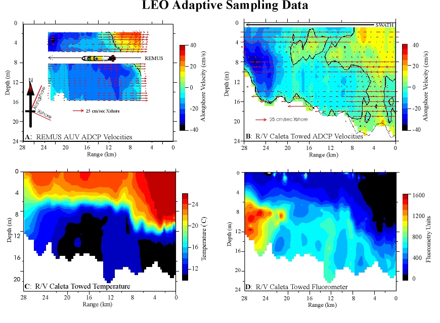
Figure 9: LEO adaptive sampling data.Top: (A & B) Alongshore (color contours) and cross-shore (arrows) velocity components derived from the upward and downward looking ADCPs on the REMUS Survey AUV (A) and the downward looking ADCP on the surface-towed SWATH (B). A northward flowing surface jet is observed offshore, and a southward flowing subsurface jet is observed inshore.
Bottom: Temperature (C) and Fluorometer (D) sections obtained from the towed undulator. The offshore jet is located in the warm, clear water above the thermocline, and the nearshore jet is located in the cold, phytoplankton rich water below the thermocline.